Understanding Selection Bias

Measuring the effect of an intervention, or ‘treatment’, is essential to the scientific method. It helps us to separate real relationships from spurious ones. But there are some pitfalls that cloud our ability to see the true effects of a treatment.

Let’s try to understand these pitfalls using an explicit example. Suppose that we want to test the impact of a new fangled weight loss pill that has been released in only one town. The pill was only available at one particular stall and people had to take it there and then.

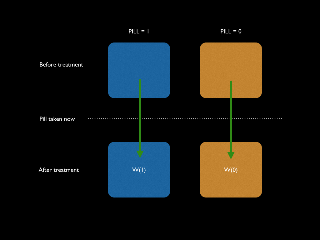
We cannot control who took the pill and who didn’t, but we do know who took it. So, we can split the population up into two groups. Let’s call them PILL = 1 if they took the pill, and PILL = 0 if they didn’t take it. We can draw a simple diagram to show this:

The blue people are those that took the pill, and the orange are those that didn’t. We can measure the outcomes of people that took the pill, call this W(1); and the outcomes of those who didn’t, call this W(0). The outcome here could be weight loss, for example.

Let’s consider for a minute what we would ideally like to know in order to examine the effects of the pill. If we took a guy from the blue group, to measure the exact impact the pill had, we would have to compare the difference between W(1) and W(0) for that same individual. But obviously, it is not possible to view the same person in two different states at the same time. The case where the blue guy’s weight loss was observed without having taken the pill is more formally denoted by [W(0) | PILL = 1].¹The ‘|’ symbol means ‘given’. This is known as a counterfactual outcome, because it never happened and so we can never directly measure it. It is represented by the right-diagonal arrow in the diagram below.

Similarly, for a person in the orange group, who never had the pill, it is impossible to observe their weight loss in the case that they had taken the pill: [W(1) | PILL = 0]. This is the effect denoted by the left-diagonal arrow.

Selection Bias

How do we measure the effectiveness of the pill? The simplest thing that we can do is to average out the weight loss for the pill takers E[W(1)], and subtract the average weight loss for the non-pill takers E[W(0)]. This would give us a form of ‘average treatment effect’ (ATE):

ATE = E[W(1) – W(0)]

= E[W(1) | PILL = 1] – E[W(0) | PILL = 0]

What’s the problem with this measure? If the individuals were randomly chosen to take the pill, then this is exactly what we want. This is because there is no systematic bias in other variables individuals might have within each group. But if they are not randomly chosen, as we assume in this case, then our problem is that the people who chose to take the pill may have some predisposition that led them to choose the pill in the first place. In other words, the blue people may have a higher (or lower) propensity to lose weight than the orange people anyway. Hence, we aren’t really capturing effects of the pill, but the effects of the pill and underlying group differences.

Remember what we would really like to know is what would have happened to the blue guys if they hadn’t taken the pill so then we could compare that to what we observed if they had taken the pill. What we want is the ‘average treatment effect on the treated’ or ATT:

ATT = E[W(1) | PILL = 1] – E[W(0) | PILL = 1]

The second term in that expression is the counterfactual that we cannot observe. So how does this relate to what we can measure? Well, take the ATE expression that we had before:

ATE = E[W(1) | PILL = 1] – E[W(0) | PILL = 0]

Now we can just add and subtract the counterfactual term to the right hand side (so that the expression is unchanged):

ATE = E[W(1) | PILL = 1] – E[W(0) | PILL = 0] + E[W(0) | PILL = 1] – E[W(0) | PILL = 1]

ATE = { E[W(1) | PILL = 1] – E[W(0) | PILL = 1] } + { E[W(0) | PILL = 1] – E[W(0) | PILL = 0] }

Now, the bit in the first curly brackets is what we want, our ATT. The bit in the second curly brackets is called selection bias. Hence:

ATE = ATT + Selection Bias

This tells us that what we actually see (ATE) is what we want (ATT) plus a term which represents the inherent differences between the blue and orange people – the selection bias.

How do we deal with this?

Randomisation when assigning people to treatments is really important, and you’ll hear this stressed a lot in scientific experiments. Random assignment means that in a large enough sample, the selection bias term will be zero. This is because the selection bias term represents the difference in weight losses between the blue people and orange people after not taking the pill:

Selection Bias = E[W(0) | PILL = 1] – E[W(0) | PILL = 0]

As I mentioned before, if the blue and orange groups were randomly chosen, then there would be no systematic difference between the average ability of a blue person to lose weight and the average ability of an orange person to lose weight. Therefore, in a situation where you have control, you always want to randomise in order to get an accurate measure of the effects.

However, in our example, people just chose to take the pill or not to by themselves. This represents much of the reality in economics, and related disciplines that involve analysis of treatments that have not been randomly assigned (i.e. by using pre-existing data). In these settings, the issue of finding a real treatment effect becomes much more difficult, and this is why econometric tools need to be quite advanced.