If you ever encounter some data in your life, you’re likely to come across a scatter diagram, which plots two variables against each other. You’re also quite likely to see a ‘line of best fit’ going through those points, which describes the apparent trend or correlation between the two variables, as suggested by the data points you’ve observed.
It’s quite possible that in your early school days, you had to draw a line of best fit through some data by eye, with a pencil and ruler. Not necessarily a bad way to do it, but it’s not going to be the optimal line every time (unless you’re extremely lucky). Of course, these days, you can just ask a computer program to do it for you – no doubt many of you have used the ‘add trendline’ feature in MS Excel.
Depending on how advanced your mathematics/statistics education is, you may have drawn a ‘line of best fit’ (or regression line) using a formula. This formula gives you an easy way of working out the exact slope and intercept of your regression line, given information about the data you’ve collected. But have you ever wondered why this works? Where does this magical formula come from?
Some Terminology

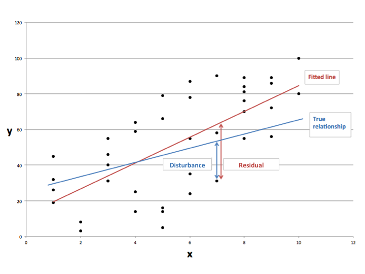
I cooked up a graph to help you understand some of the things that I’ll be talking about. Firstly, we call y the regressand (or dependent variable) and x the regressor (or independent variable). This means that given some value of x, we want to see how the value of y depends on it.
If it helps, you can give x and y names. For example, x could represent years of experience at knitting socks, and y could represent the overall quality of sock produced by a particular granny. Each point on the graph represents the experience and output quality information of a specific granny.
Here’s where it gets interesting. There must be some underlying true relationship between x and y (it could be that there is no relationship, but that still counts). We don’t know what that true relationship is, because we only have a sample of n data points. Or, we don’t know the real relationship between years of granny’s knitting and quality of sock, because we can’t track down every single granny in the world that knits. That true relationship could be linear, or it could be something far more complicated. However, suppose I have magical powers and actually know the true relationship in this instance. I’ve represented that with a blue line.
Of course, not every point lies on that line. This is because there are probably other factors which we can’t observe that cause a ‘disturbance’ to the data. Your granny’s knitting ability may not only depend on years spent knitting, she may have had joint replacements that affect her motor skills or she may have inherited an instinctive genetic ability to perform a cross-stitch. Either way, the difference between the actual data observations and the true relationship is known as the disturbance (or error) term.
Let’s denote the disturbances of the true line as ε, the intercept (where it crosses the vertical axis) α and the slope of the line β. Then, for each observation i=1,2,…,n (or each granny), the true relationship between x and y is given by:
\[y_i = \alpha + \beta x_i + \epsilon_i \]
The equation of the true line is given by the first two terms on the right hand side. The disturbances are what takes us off the line and to a particular data point.
Now, as I said before, in reality, we wouldn’t know what the true relationship was. We wouldn’t know the ‘true line’, so we have to estimate it. This is what we call the ‘line of best fit’ or regression line.
In the graph, the fitted line is in red. As you can see, the line is a bit different to the true line, but this is because we are working from a sample and don’t have all the data. The fitted line allows us to predict, on average, what we can expect y to be given an x value. In terms of grannies, our line tells us that for a granny with p years of knitting experience, we can predict that she will produce socks of quality q. The equation for our fitted line is:
\[\hat{y}_i = \hat{\alpha} + \hat{\beta} x_i \]
The ‘hat’ symbol on the letters means that they are estimates of the true values. Of course, if we wanted to get the actual data points, we’d have to move off the line. The distance that we move off the line is known as a residual. The residual is basically an estimate of the disturbance term, and so it’s not quite the same as the disturbance itself. So, to get the original value of y, we must add on our residuals to the fitted line for each observation i:
\[y_i = \hat{\alpha} + \hat{\beta} x_i + \hat{\epsilon_i}\]
How can we draw a line that fits the data best? There are many ways of doing it, but the general idea is always the same. We want to try to draw the line so that we minimise the distance between our line and all the data points that we have. This, by definition, will be the line that best fits the data. The method we will use is the most common one, the method of least squares, invented by Gauss in the 18th century.
The idea is this: to get the line as close to all the data points as possible, we want to minimise the residuals. However, if we just add up the residuals, they’ll cancel each other out, because some will be positive (when the data point is above the fitted line) and others will be negative (when the point is below the fitted line). So we instead take the squares of the residuals and minimise the sum of them all. Nice neat idea.
In summary then, what we need are estimates for α and β such that the residual sum of squares (RSS) is minimised. All of a sudden, our problem has become a 2-variable optimisation problem, and so we can use calculus to solve it.
Deriving the Ordinary Least Squares (OLS) Estimators
The thing we want to minimise is the RSS, which is:
\[\sum\limits_{i=1}^n \hat{\epsilon_i^2} = \sum\limits_{i=1}^n (y_i – \hat{\alpha} – \hat{\beta} x_i )^2\]
Here, I’ve just substituted for ε by rearranging the previous fitted equation. We can continue simplifying by explicitly squaring what’s inside the brackets:
\[= \sum\limits_{i=1}^n (y_i^2 + \hat{\alpha}^2 + \hat{\beta}^2 x_i^2 – 2\hat{\alpha} y_i – 2 \hat{\beta} x_i y_i + 2\hat{\alpha} \hat{\beta} x_i^2)\]
\[= \sum\limits_{i=1}^n y_i^2 + n\hat{\alpha}^2 + \hat{\beta}^2 \sum\limits_{i=1}^n x_i^2 – 2n \hat{\alpha} \bar{y} – 2 \hat{\beta} \sum\limits_{i=1}^n x_i y_i + 2n\hat{\alpha} \hat{\beta} \bar{x}\]
Note that to simplify, I’ve used some shorthand to represent the sample means of x and y:
\[\frac{1}{n} \sum\limits_{i=1}^n y_i = \bar{y}, \frac{1}{n} \sum\limits_{i=1}^n x_i = \bar{x}\]
To minimise the expression for RSS that we’ve obtained, we partially differentiate with respect to the variables we want to get optimal values for:
\[\frac{\partial RSS}{\partial \hat{\alpha}} = 0 \Leftrightarrow 2n\hat{\alpha} – 2n\bar{y} + 2n\hat{\beta} \bar{x} = 0\]
\[\frac{\partial RSS}{\partial \hat{\beta}} = 0 \Leftrightarrow 2\hat{\beta} \sum\limits_{i=1}^n x_i^2 – 2\sum\limits_{i=1}^n x_i y_i + 2n \hat{\alpha} \bar{x} = 0\]
The first simplifies nicely to give us the expression for the OLS estimator of α:
\[\hat{\alpha} = \bar{y} – \hat{\beta} \bar{x}\]
The second requires a little more fiddling:
\[\hat{\beta} \sum\limits_{i=1}^n x_i^2 = \sum\limits_{i=1}^n x_i y_i – \hat{\alpha}n \bar{x}\]
Substituting for α:
\[\hat{\beta} \sum\limits_{i=1}^n x_i^2 = \sum\limits_{i=1}^n x_i y_i – (\bar{y} – \hat{\beta} \bar{x}) n \bar{x}\]
Rearranging:
\[\hat{\beta} = \frac{ \sum\limits_{i=1}^n x_i y_i – n \bar{x}\bar{y} }{\sum\limits_{i=1}^n x_i^2 – n\bar{x}^2}\]
Or equivalently (and a bit more neatly):
\[\hat{\beta} = \frac{ \sum\limits_{i=1}^n (x_i – \bar{x})(y_i – \bar{y}) }{\sum\limits_{i=1}^n (x_i – \bar{x})^2}\]
And so, we’re done! We now have the OLS estimators for the case where there is one regressor. This analysis can be extended to allow for any number of regressors with the use of vectors and matrices, but I won’t go into this here since I think we’ve done enough for one day. Happy line drawing!
I would like to express my love of this article in the following manner:
(sqrt(cos(x))*cos(400*x)+sqrt(abs(x))-0.4)*(4-x*x)^0.1
Thanks 😉
Thank you so much! This became very much helpful for my assignment work.